Article Highlights
- To randomly sample rows in R, you can use the Base R approach by sampling row indices, or the dplyr approach for a more readable syntax.
- Base R:
df[sample.int(nrow(df), size = 10), ]selects 10 random rows. - dplyr:
df |> slice_sample(n = 10)achieves the same result. - Reproducibility: Always use
set.seed()before sampling to ensure your results are consistent.

Note: This blog assumes you are using the R Programming Language in RStudio Desktop.
It is impossible to imagine a data scientist who does not need to randomly sample datasets on a regular basis. Whether you are bootstrapping, creating mini-batches for machine learning, or simply exploring a massive dataset, you need efficient tools. Below, we explore the classic sample() function and modern alternatives like slice_sample() that are standard in 2026.
Using Base R: The sample() Function
The sample() function serves as the foundation for random sampling in R. While traditionally used on vectors, we apply it to dataframes by generating row indices and subsetting.
Basic Usage: Sampling Rows
For robust production code, we recommend sample.int() over the standard sample(). While both work, sample.int() explicitly treats its first argument as a number of items, avoiding edge-case bugs that can occur with single-row datasets.
# Basic syntax for sampling 30 rows without replacement

# sample.int() is the safer, explicit alternative to sample()
iris.sampled <- iris[sample.int(nrow(iris), 30), ]
To clarify, here is a step-by-step breakdown:
- Count rows:
nrow(iris)gets the total number of rows. - Sample indices:
sample.int(nrow(iris), 30)picks 30 random numbers between 1 and the total row count. - Subset:
iris[..., ]uses those numbers to grab the specific rows.
Note: For vector columns, you can sample values directly: sample(iris[, "Sepal.Length"], 30).
Sampling Without Replacement
Sampling without replacement ensures each row appears at most once in your sample—ideal for test/train splits or bootstrapped partitions where overlap isn't desired.
# Sample 10 rows without replacement

# replace = FALSE is the default for sample.int, but being explicit helps readability
sampled_without_replacement <- iris[sample.int(nrow(iris), 10), ]
Sampling With Replacement
Sampling with replacement enables duplicate rows in the sample, allowing any row to be drawn multiple times. This is essential for techniques like bootstrapping and bagging in ensemble learning workflows.
# Sample 10 rows with replacement (duplicates possible)
sampled_with_replacement <- iris[sample.int(nrow(iris), 10, replace = TRUE), ]| Scenario | Replace Argument | Result |
|---|---|---|
| Without replacement | FALSE | No duplicate rows selected |
| With replacement | TRUE | Rows can appear multiple times |
Understanding these distinctions empowers you to design sampling strategies fitting any analytical workflow.
The dplyr Approach: slice_sample()
In modern R programming, the tidyverse offers a more intuitive syntax. While you may see older code using sample_n(), this has been superseded by slice_sample().
library(dplyr)

# Select 10 random rows
df |> slice_sample(n = 10)

# Select 50% of the rows
df |> slice_sample(prop = 0.5)
slice_sample() handles the row index logic internally, making your code cleaner and easier to read.
Weighted Sampling
Sometimes not all rows are created equal. If you need to sample rows based on specific weights (e.g., giving recent transactions a higher probability of being chosen), slice_sample makes this easy with the weight_by argument.
# Weighted sampling: Give rows with larger Sepal.Length a higher chance of selection
iris |> slice_sample(n = 10, weight_by = Sepal.Length)
A Direct "Hands-On" Approach: Logical Vectors
We don't actually need the sample() function to select indices. A direct approach using logical vectors can offer flexibility if you require a customized probability distribution. Let's look at rbinom(), one of R's random number generators.
The following example generates the numerical equivalent of tossing four pennies, recording the number of heads, and repeating the experiment 50 times:
rbinom(50, 4, 0.5)If we are sampling rows, we only want the equivalent of one penny flip per row. Heads we take the row (TRUE); tails we leave it behind (FALSE).
Creating the Logical Vector
We need a logical vector (TRUE/FALSE) the same length as our dataframe. Here is how to select approximately 10% of the rows using a binomial distribution:
# Create a logical vector where each row has a 10% chance of being TRUE
logical_selection <- as.logical(rbinom(nrow(iris), 1, 0.10))

# Subset the dataframe
subset_df <- iris[logical_selection, ]
Why usage of nrow() matters: Older code samples might use length(df[[1]]) to get the row count. Using nrow(df) is safer and more standard.
Console Output:
| Row | Sepal.Length | Sepal.Width | Petal.Length | Petal.Width | Species |
|---|---|---|---|---|---|
| 17 | 5.4 | 3.9 | 1.3 | 0.4 | setosa |
| 27 | 5.0 | 3.4 | 1.6 | 0.4 | setosa |
| 30 | 4.7 | 3.2 | 1.6 | 0.2 | setosa |
| 43 | 4.4 | 3.2 | 1.3 | 0.2 | setosa |
| 44 | 5.0 | 3.5 | 1.6 | 0.6 | setosa |
| 59 | 6.6 | 2.9 | 4.6 | 1.3 | versicolor |
| 82 | 5.5 | 2.4 | 3.7 | 1.0 | versicolor |
| 97 | 5.7 | 2.9 | 4.2 | 1.3 | versicolor |
| 106 | 7.6 | 3.0 | 6.6 | 2.1 | virginica |
| 118 | 7.7 | 3.8 | 6.7 | 2.2 | virginica |
Splitting a Dataframe into Training and Testing Sets
A fundamental step in supervised machine learning is dividing your dataset into training and testing subsets. This separation allows you to fit your model on one portion of the data (training) and evaluate its performance on another (testing), ensuring unbiased estimates of predictive accuracy.
Logical Vector Method for Data Splitting
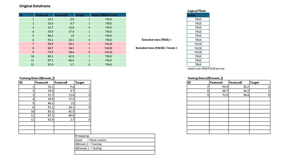
In R, you can construct a logical vector to specify which rows belong in the training set (TRUE) and which in the testing set (FALSE).
# Set seed for reproducibility
set.seed(123)

# Create a logical vector: 80% TRUE (training), 20% FALSE (testing)
# Note: This is a probabilistic split; exact counts may vary slightly.
random_logical_vector <- sample(c(TRUE, FALSE), nrow(iris), replace = TRUE, prob = c(0.8, 0.2))

# Subset training and testing sets
training <- iris[random_logical_vector, ]
testing  <- iris[!random_logical_vector, ]
This approach guarantees that each row is assigned to exactly one bucket—either training or testing—with probabilities you control. The logical vector is mapped directly to the rows of your dataframe.
For complex tasks, such as stratified sampling to preserve group proportions, consider specialized packages like rsample and its initial_split() function.
Bootstrapped Datasets and Applications in Machine Learning
Bootstrapping is a fundamental resampling technique in statistical learning, where you sample rows with replacement to create multiple datasets. This process is essential for estimating model accuracy, generating confidence intervals, and building ensemble models like bagged trees and random forests.
Creating Bootstrapped Samples in R
To generate a bootstrapped dataset from your original dataframe, set the replace argument to TRUE in the sample() function. The resulting bootstrapped sample has the same number of rows as your original data but may include duplicates.
# Bootstrapped sampling: sample n rows with replacement
boot_indices <- sample.int(nrow(iris), nrow(iris), replace = TRUE)
bootstrapped_iris <- iris[boot_indices, ]
Example: Bagged Trees
Bagging (Bootstrap Aggregating) involves fitting multiple decision trees to different bootstrapped samples and aggregating their predictions.
library(ipred)
set.seed(42)
bagged_model <- bagging(Species ~ ., data = iris, nbagg = 25)
Example: Random Forests
Random forests extend the bagging concept with additional randomness during tree construction.
library(randomForest)
set.seed(42)
rf_model <- randomForest(Species ~ ., data = iris, ntree = 100)
Bootstrapped datasets not only improve model robustness but also provide reliable measures of uncertainty. For further reading on ensemble methods and the theory behind bootstrapping, consult the CRAN Task View on Machine Learning.
Stratified Sampling in R
Random sampling is a foundational tool for data science workflows, but there are many situations—such as highly imbalanced datasets—where uniform random selection may not produce representative subsets. Stratified sampling addresses this issue by ensuring each subgroup (stratum) in your data is proportionally represented in the resulting samples. This is common when building training and testing datasets for classification problems.
Why Use Stratified Sampling?
Without stratification, you might accidentally exclude rare or minority classes from your training or testing set. This can result in biased models with poor performance on underrepresented classes. By stratifying, you preserve the statistical properties of your target variable (e.g., species or class membership), leading to more reliable model evaluation and generalizability.
Example: Stratified Train/Test Split with rsample
The rsample package provides a robust and reproducible approach to stratified sampling. Here’s how to implement an 80/20 stratified split on the classic iris dataset by species:
library(rsample)

# Set a reproducible seed
set.seed(123)

# Perform the stratified split
split <- initial_split(iris, strata = "Species", prop = 0.8)

# Extract training and testing sets
training_set <- training(split)
testing_set <- testing(split)

# Confirm the distribution is stratified
prop.table(table(training_set$Species))
prop.table(table(testing_set$Species))
In this example, the proportion of each species in both training and testing sets closely matches the overall dataset distribution, making this a best practice for supervised learning.
Ready to enhance your data sampling skills even further? Try this Hands-on Introduction to R course from Learning Tree International!
Frequently Asked Questions
How do I sample rows with replacement in R?
To sample with replacement (where the same row can be selected more than once), set the replace argument to TRUE.
In Base R: sample.int(nrow(df), size, replace = TRUE).
In dplyr: slice_sample(df, n = size, replace = TRUE).
What is the difference between sample_n() and slice_sample()?
sample_n() is an older dplyr function that has been superseded. slice_sample() is the modern alternative that provides a consistent interface with other slice functions and avoids inconsistencies with grouped dataframes.
Why should I use set.seed() when sampling?
R generates "pseudo-random" numbers. Using set.seed(123) (or any integer) initializes the random number generator to a specific point, ensuring that your code produces the exact same random sample every time it is run. This is critical for reproducible research.
What do I do with this new dataset? How can I learn more?
There are two related courses that would pair well with new sampling skills:
Introduction to AI, Data Science & Machine Learning with Python
While the blog uses R, the section on "Bootstrapped Datasets and Applications in Machine Learning" touches on universal concepts like Random Forests and Bagging. This course is an excellent pairing because it broadens your data science toolkit. It covers the same machine learning concepts (training/testing, ensemble methods) but introduces you to Python, allowing you to become a bilingual data scientist—a highly standard requirement in 2026.
Introduction to Power BI Training
Once you have sampled and analyzed your datasets using the techniques in the blog (like stratified sampling), the next logical step is visualization and reporting. Power BI integrates well with R scripts, allowing you to take the sampled datasets you created in R and visualize them in interactive dashboards for stakeholders.
This blog was updated in February 2026 with updated information on the tidyverse and rsample packages.